Fred's Flare Formula
Alignments to Content Standards:
S-IC.B.4
Task
Roadside flares are often used by motorists to warn oncoming drivers of obstacles in the roadway and to draw attention to hazardous road conditions. Generally, flares are small and portable. One of the great conveniences of the flares is that they do not require electricity. The light from the flare is caused by a chemical reaction from elements inside the flare, and they can be used in many conditions.
Fred’s Flare Company made flares that burned for 100 minutes on average. However, Fred has developed a new chemical process that should allow the flares to now burn slightly over 120 minutes (that is, over 2 hours) on average; and the claim of “Now burns for over 2 hours on average” will be stated on the packages in which the new flares are sold.
Because of this claim on the package, the company must periodically sample a group of flares and check to see if the “Now burns for over 2 hours on average” claim is reasonable for the population of all flares they manufacture.
1. If every manufactured flare was sampled, that would be called a census, and the population average burn time could be computed directly. Give at least one reason why a census would not be feasible in this case.
Random Sampling
If random sampling is used, it is reasonable for Fred to use the mean burning time of a given sample (a sample mean) to estimate the mean burning time of his entire population (the population mean). Knowing that there is variability in all manufacturing, Fred knows that even if the mean burn time of all of the flares is actually over 120 minutes on average, he could occasionally get a sample with an average burn time that is not over 120 minutes. However, he also wants to be confident that a population mean burning time of over 120 minutes is plausible.
Even though Fred’s company will manufacture several thousand flares each day, sampling is somewhat costly, so Fred wants to sample as few flares as possible. Previously, when the old “100 minute” flares were tested, the company would take a sample of 20 flares each hour from the production line and compute a mean burning time for each sample of 20 flares. Fred determines that this sampling method should continue for the new flares. The results of one full day of this hourly testing are shown below. (One day = 24 hourly samples, so 24 sample means shown in the dotplot.)
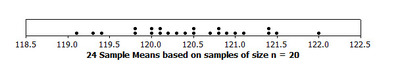
2. According to the dotplot, how many of these 24 sample averages are at or below 120 minutes? What percentage of these 24 sample averages are at or below 120 minutes? What percentage of the samples are strictly below 120 minutes?
3. By visual inspection of the dotplot, estimate the values in the 5-number summary for these 24 hourly sample averages. What is the range of these 24 sample average measurements?
The big question for Fred is: do the results of this day's sampling raise concern about the “Now burns for over 2 hours on average” claim?
4. Use the dotplot and/or the analysis you've performed above to address Fred's question. Be thorough and mention any information that seems to support the “Now burns for over 2 hours on average” claim and any information that would not encourage you to support that claim. In one sentence, what will you tell Fred? Are you confident that that the population mean burning time is more than 120 minutes?
A Larger Sample Size
Fred is concerned by the results, but he is still fairly sure that the population average burning time is slightly more than 120. He decides to sample 100 flares every hour instead of just 20. A dotplot showing the averages from the 24 samples of size 100 from this second day of sampling is as follows:

Keep in mind that the MANUFACTURING PROCESS DID NOT CHANGE, only the sample size for the hourly sampling was changed -- specifically it was increased to 5 times its original size (from 20 flares to 100 flares per sample).
Now re-examine the previous questions using this new dotplot.
5. According to this NEW dotplot, how many of the 24 sample averages are at or below 120 minutes?
6. By visual inspection of the dotplot, estimate the values in the 5-number summary for these 24 NEW sample averages. What is the range of these 24 sample averages?
7. Using this NEW dotplot that came from sampling that used a larger sample size and the analysis you've just performed, what general information about these 24 sample averages seems to support the claim that the population mean burning time is more than 120 minutes?
Comparing the Dotplots and the Sample Sizes
8. Which distribution of the 24 hourly averages had the smaller range: the distribution of sample averages based on a sample of size 20, or the distribution of sample averages based on a sample of size 100?
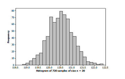
To further examine the effect of sample size, consider the following histograms representing two sampling simulations from the same flare population. In the first simulation, we imagine that Fred continued to take random samples of size 20 every hour for 30 days. In the second simulation, we imagine that Fred continued to take random samples of size 100 every hour for 30 days. Note: both distributions represent the averages from 720 samples (720 = 24 hours * 30 days).

9. Assuming that the cost to sample 100 flares per hour is only slightly more than the cost to sample 20 flares per hour, would you recommend using a larger sample size or a smaller sample size to estimate the population mean? Explain.
Margin of Error
In the dotplots given earlier, each dot represented a sample mean and each sample mean is an estimate of the population mean burning time. When random sampling is used, in the long run, sample means generated from many random samples tend to be centered around the actual population mean. For example, here are the averages of the four distributions shown above:
When the sample was size 20, the average of the 24 hourly sample means = 120.46 minutes
When the sample was size 100, the average of the 24 hourly sample means = 120.49 minutes
When the sample was size 20, the average of the 720 hourly sample means = 120.50 minutes
When the sample was size 100, the average of the 720 hourly sample means = 120.50 minutes
In other words, the “average of all the sample averages” in all 4 cases was about 120.5 minutes (rounded). That would be a good estimate for the population mean burning time. Unfortunately, in most cases, you don’t collect many random samples—you only select one random sample for analysis.
A margin of error is loosely defined as the largest expected size of the difference between an estimate and the actual population value that is being estimated. For example, if you were trying to estimate the average weight of a population based on a proper sample and your margin of error was stated as "2 pounds," that is saying that you would be very confident that the actual population mean weight is within 2 pounds of your sample estimate. In other words, if you obtained a sample average weight of 45 pounds and your margin of error was 2 pounds, you would be very confident that the actual population mean weight would be somewhere between 43 pounds (that's 45 – 2 pounds) and 47 pounds (that's 45 + 2 pounds).
One informal way of developing a margin of error from a simulation is to compute the midrange (= range/2) of the simulations results. For the first simulation histogram (the one based on samples of size n = 20), this informal margin of error value would be roughly 1.8 minutes (you can confirm this above). If the true population mean was in fact 120.5 minutes, that value would be within the margin of error of every one of the 720 estimates. In other words, no matter which one of the 720 estimates you selected, the value "120.5 minutes" would be within 1.8 minutes of that estimate.
10. If we perform this same informal method of developing a margin of error using the second simulation histogram (the one based on samples of size n = 100), what would the value for the margin of error be?
11. Generally speaking, do you think that when proper random sampling occurs, the margin of error for estimating a population mean gets smaller or larger as the sample size increases?
IM Commentary
Although margin of error can be computed by formula, this task is intended to engage students into considering how it can be estimated from examining the results of repeated simple random sampling. This approach should also assist students in developing a more visual sense as to what “margin of error” means in terms of estimation.
A key point for students to address up front is that even perfect simple random sampling will not usually yield a sample estimate that is equal to the value of the population parameter it is estimating. There will always be some sampling variability in a case like the one in this task. However, students should also realize that using larger samples (properly collected) leads to less sampling variability and thus a smaller margin of error when estimating the parameter.
Solution
1. Hopefully students will realize that if every flare were burned to determine its burn time, no flares would be left to sell. Comments regarding the large cost and time involved in a full census are on the right track, but this is a particular case where the sampled items are in fact used up while being tested.
2. Seven of the 24 sample averages are at or below 120 minutes (7/24 = 29.17%). Five of the 24 sample averages are strictly below 120 minutes (5/24 = 20.83%).
3. Actual values:
Minimum Q1 Median Q3 Maximum
119.06 120.00 120.42 120.95 122.04
Range almost 3 minutes (2.98 minutes)
Student answers should be close to these values but may not be quite this precise since the actual data values are not presented.
4. Support: Almost 71% of the sample averages are above 120 minutes. (A reference to Q1 = 120 minutes or the fact that the median is higher than 120 minutes could also be good points to mention.) Against: Almost 30% of the sample averages are less than or equal to 120 minutes. It would be hard to confidently support a claim that the population average is over 120 minutes with that many low values in a day's sampling.
5. None of the 24 sample averages are at or below 120 minutes.
6. Actual values:
Minimum Q1 Median Q3 Maximum
120.03 120.34 120.52 120.63 120.95
Range less than 1 minute (0.92 minutes)
7. Since all 24 sample averages are above 120 minutes, there is good evidence that the population average which is being estimated is also above 120 minutes.
8. Using samples of size 100 made for a distribution with a smaller range. The sample averages didn’t vary as widely.
9. The larger sample sizes are yielding estimates that do not vary as much. The larger sample size is preferable if it is affordable.
10. The midrange can be used to estimate the margin of error. It is roughly 0.7 minutes
11. Generally, the margin of error would decrease as sample size increases.
Fred's Flare Formula
Roadside flares are often used by motorists to warn oncoming drivers of obstacles in the roadway and to draw attention to hazardous road conditions. Generally, flares are small and portable. One of the great conveniences of the flares is that they do not require electricity. The light from the flare is caused by a chemical reaction from elements inside the flare, and they can be used in many conditions.
Fred’s Flare Company made flares that burned for 100 minutes on average. However, Fred has developed a new chemical process that should allow the flares to now burn slightly over 120 minutes (that is, over 2 hours) on average; and the claim of “Now burns for over 2 hours on average” will be stated on the packages in which the new flares are sold.
Because of this claim on the package, the company must periodically sample a group of flares and check to see if the “Now burns for over 2 hours on average” claim is reasonable for the population of all flares they manufacture.
1. If every manufactured flare was sampled, that would be called a census, and the population average burn time could be computed directly. Give at least one reason why a census would not be feasible in this case.
Random Sampling
If random sampling is used, it is reasonable for Fred to use the mean burning time of a given sample (a sample mean) to estimate the mean burning time of his entire population (the population mean). Knowing that there is variability in all manufacturing, Fred knows that even if the mean burn time of all of the flares is actually over 120 minutes on average, he could occasionally get a sample with an average burn time that is not over 120 minutes. However, he also wants to be confident that a population mean burning time of over 120 minutes is plausible.
Even though Fred’s company will manufacture several thousand flares each day, sampling is somewhat costly, so Fred wants to sample as few flares as possible. Previously, when the old “100 minute” flares were tested, the company would take a sample of 20 flares each hour from the production line and compute a mean burning time for each sample of 20 flares. Fred determines that this sampling method should continue for the new flares. The results of one full day of this hourly testing are shown below. (One day = 24 hourly samples, so 24 sample means shown in the dotplot.)
2. According to the dotplot, how many of these 24 sample averages are at or below 120 minutes? What percentage of these 24 sample averages are at or below 120 minutes? What percentage of the samples are strictly below 120 minutes?
3. By visual inspection of the dotplot, estimate the values in the 5-number summary for these 24 hourly sample averages. What is the range of these 24 sample average measurements?
The big question for Fred is: do the results of this day's sampling raise concern about the “Now burns for over 2 hours on average” claim?
4. Use the dotplot and/or the analysis you've performed above to address Fred's question. Be thorough and mention any information that seems to support the “Now burns for over 2 hours on average” claim and any information that would not encourage you to support that claim. In one sentence, what will you tell Fred? Are you confident that that the population mean burning time is more than 120 minutes?
A Larger Sample Size
Fred is concerned by the results, but he is still fairly sure that the population average burning time is slightly more than 120. He decides to sample 100 flares every hour instead of just 20. A dotplot showing the averages from the 24 samples of size 100 from this second day of sampling is as follows:
Keep in mind that the MANUFACTURING PROCESS DID NOT CHANGE, only the sample size for the hourly sampling was changed -- specifically it was increased to 5 times its original size (from 20 flares to 100 flares per sample).
Now re-examine the previous questions using this new dotplot.
5. According to this NEW dotplot, how many of the 24 sample averages are at or below 120 minutes?
6. By visual inspection of the dotplot, estimate the values in the 5-number summary for these 24 NEW sample averages. What is the range of these 24 sample averages?
7. Using this NEW dotplot that came from sampling that used a larger sample size and the analysis you've just performed, what general information about these 24 sample averages seems to support the claim that the population mean burning time is more than 120 minutes?
Comparing the Dotplots and the Sample Sizes
8. Which distribution of the 24 hourly averages had the smaller range: the distribution of sample averages based on a sample of size 20, or the distribution of sample averages based on a sample of size 100?
To further examine the effect of sample size, consider the following histograms representing two sampling simulations from the same flare population. In the first simulation, we imagine that Fred continued to take random samples of size 20 every hour for 30 days. In the second simulation, we imagine that Fred continued to take random samples of size 100 every hour for 30 days. Note: both distributions represent the averages from 720 samples (720 = 24 hours * 30 days).
9. Assuming that the cost to sample 100 flares per hour is only slightly more than the cost to sample 20 flares per hour, would you recommend using a larger sample size or a smaller sample size to estimate the population mean? Explain.
Margin of Error
In the dotplots given earlier, each dot represented a sample mean and each sample mean is an estimate of the population mean burning time. When random sampling is used, in the long run, sample means generated from many random samples tend to be centered around the actual population mean. For example, here are the averages of the four distributions shown above:
When the sample was size 20, the average of the 24 hourly sample means = 120.46 minutes
When the sample was size 100, the average of the 24 hourly sample means = 120.49 minutes
When the sample was size 20, the average of the 720 hourly sample means = 120.50 minutes
When the sample was size 100, the average of the 720 hourly sample means = 120.50 minutes
In other words, the “average of all the sample averages” in all 4 cases was about 120.5 minutes (rounded). That would be a good estimate for the population mean burning time. Unfortunately, in most cases, you don’t collect many random samples—you only select one random sample for analysis.
A margin of error is loosely defined as the largest expected size of the difference between an estimate and the actual population value that is being estimated. For example, if you were trying to estimate the average weight of a population based on a proper sample and your margin of error was stated as "2 pounds," that is saying that you would be very confident that the actual population mean weight is within 2 pounds of your sample estimate. In other words, if you obtained a sample average weight of 45 pounds and your margin of error was 2 pounds, you would be very confident that the actual population mean weight would be somewhere between 43 pounds (that's 45 – 2 pounds) and 47 pounds (that's 45 + 2 pounds).
One informal way of developing a margin of error from a simulation is to compute the midrange (= range/2) of the simulations results. For the first simulation histogram (the one based on samples of size n = 20), this informal margin of error value would be roughly 1.8 minutes (you can confirm this above). If the true population mean was in fact 120.5 minutes, that value would be within the margin of error of every one of the 720 estimates. In other words, no matter which one of the 720 estimates you selected, the value "120.5 minutes" would be within 1.8 minutes of that estimate.
10. If we perform this same informal method of developing a margin of error using the second simulation histogram (the one based on samples of size n = 100), what would the value for the margin of error be?
11. Generally speaking, do you think that when proper random sampling occurs, the margin of error for estimating a population mean gets smaller or larger as the sample size increases?