Olympic Men's 100-meter dash
Alignments to Content Standards:
S-ID.C.7
S-ID.B.6.a
Task
The scatterplot below shows the finishing times for the Olympic gold medalist in the men's 100-meter dash for many previous Olympic games. The line of best fit is also shown. (Source: http://trackandfield.about.com/od/sprintsandrelays/qt/olym100medals.htm)
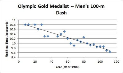
- Is a linear model a good fit for the data? Explain, commenting on the strength and direction of the association.
- The equation of the linear function that best fits the data (the line of best fit) is $$\widehat{\mbox{Finishing time}} = 10.878 - 0.0106 \left( \mbox{Year after 1900} \right).$$ Given that the summer Olympic games only take place every four years, how should we expect the gold medalist's finishing time to change from one Olympic games to the next?
- What is the vertical intercept of the function's graph? What does it mean in context of the 100-meter dash?
- Note that the gold medalist finishing time for the 1940 Olympic games is not included in the scatterplot. Use the model to estimate the gold medalist's finishing time for that year.
- What is a realistic domain for the linear function? Comment on how your answer pertains to using this function to make predictions about future Olympic 100-m dash race times.
IM Commentary
The task asks students to identify when two quantitative variables show evidence of a linear association, and to describe the strength and direction of that association. Students then utilize a least-squares regression line to make predictions, and to make conjectures about the limitations of the model, which is a very important aspect of SMP4 - Model with Mathematics. They must apply their knowledge of slope and intercept of a linear function in context of the problem; i.e., understand that the slope of a regression line is the predicted change in the response variable per unit change of the explanatory variable, and that the vertical intercept corresponds to a value of zero in the explanatory variable.
Linear models are a very nice connection between statistics and functions in high school mathematics. Coherence in high school mathematics means drawing connections between topics that use the same mathematical concept. In this case we use linear functions to model the relationship between two quantitative variables. We can use the context of investigating if there is an association between two variables to strengthen our understanding of slope and intercept of a linear function.
This task is probably most appropriate for use in instruction. Consider having students work together in pairs or small groups on parts a - d. Part e could then be the basis for a whole class discussion.
Solution
- The data in the scatterplot are from two quantitative variables (year and finishing time), and the overall pattern is linear. There are also no obvious outliers, so it is reasonable to fit a linear model to the data. The direction of the association is negative (finishing time decreases as the year after 1900 increases), and the association is strong because the points are tightly clustered in a linear form.
- The slope of the equation of the line of best fit is $-0.0106.$ This means for every 1 year that passes, we would predict that the finishing time for the 100-m dash decreases by $0.0106$ seconds. Since the Olympics take place every four years, we would expect the predicted gold medalist's finishing time to decrease by $4(0.0106) = 0.0424$ seconds from one Olympic games to the next.
- The vertical intercept of the line of best fit's equation is 10.878. In context, this would be the predicted finishing time (in seconds) for the 100-m dash gold medalist in the 1900 Olympic games.
- To predict the finishing time for the 1940 gold medalist, we would simply substitute $\mbox{Years after 1900} = 40$ into the equation of the line of best fit to solve for $\widehat{\mbox{Finishing Time}}.$ This yields $$ \widehat{\mbox{Finishing Time}} = 10.878 - 0.0106 (40) = 10.454.$$ The predicted finishing time for the 1940 gold medalist is 10.454 seconds.
- At the most basic level, we know that the model will fail to be realistic once we obtain predicted racing times of zero or less. Substituting $0$ into the equation for $\widehat{\mbox{Finishing Time}}$, we can solve for $\mbox{Years after 1900} \approx 1026.2.$ This equates to roughly the year 2926. If we take into account the current four-year rotation for the summer Olympic games, however, we see that the model will only provide a positive prediction up through the Olympic games in the year 2924. To be even more realistic, we should expect any 100-m dash to be completed in some positive amount of time; however, it may be difficult for students to put a specific value on a reasonable result. This discussion could also open up the topic of extrapolation versus interpolation when using linear models.
Olympic Men's 100-meter dash
The scatterplot below shows the finishing times for the Olympic gold medalist in the men's 100-meter dash for many previous Olympic games. The line of best fit is also shown. (Source: http://trackandfield.about.com/od/sprintsandrelays/qt/olym100medals.htm)
- Is a linear model a good fit for the data? Explain, commenting on the strength and direction of the association.
- The equation of the linear function that best fits the data (the line of best fit) is $$\widehat{\mbox{Finishing time}} = 10.878 - 0.0106 \left( \mbox{Year after 1900} \right).$$ Given that the summer Olympic games only take place every four years, how should we expect the gold medalist's finishing time to change from one Olympic games to the next?
- What is the vertical intercept of the function's graph? What does it mean in context of the 100-meter dash?
- Note that the gold medalist finishing time for the 1940 Olympic games is not included in the scatterplot. Use the model to estimate the gold medalist's finishing time for that year.
- What is a realistic domain for the linear function? Comment on how your answer pertains to using this function to make predictions about future Olympic 100-m dash race times.