Foxes and Rabbits 3

Task

Given below are two graphs that show the populations of foxes and rabbits in a national park over a 24 month period.

1. Explain why it is appropriate to model the number of rabbits and foxes as trigonometric functions of time.
2. Find an appropriate trigonometric function that models the number of rabbits, $r(t)$, as a function of time, with $t$ in months.
3. Find an appropriate trigonometric function that models the number of foxes, $f(t)$, as a function of time, with $t$ in months.

IM Commentary

The example of rabbits and foxes was introduced in 8-F Foxes and Rabbits to illustrate two functions of time given in a table. The same situation was used in F-TF Foxes and Rabbits 2 to find trigonometric functions modeling the data in the table. The previous situation was somewhat unrealistic since we were able to find functions that fit the data perfectly. In this task, on the other hand, we do some legitimate modelling, in that we come up with functions that approximate the data well, but do not perfectly match, the given data.

This task is best used for instruction. It lends itself well to students working together in groups and comparing their modeling functions. Different groups might come up with different function formulas. Students have to make several choices. They have to decide which values to use for maximum and minimum values. They also have to choose which trigonometric function to use for their model since it is possible to use positive or negative sine or cosine functions with different horizontal shifts for both populations.

Solution

1. Looking at the graphs, we notice that both populations have the basic shape of cosine and sine functions, even though there is some irregularity in the data. We can only see the data for two years, but it is reasonable to assume that the pattern will repeat itself in future years, and we are looking at periodic functions

2. To model the data with a cosine or sine function, we are looking for a function of the form $A \sin(B(t - D)) + C$ or $A \cos(B(t − D)) + C$, where $|A|$ is the amplitude, $C$ is the midline, $B = \frac{2\pi}{\text{period}}$, and $D$ is the horizontal shift. Looking at the graph, we observe that the rabbit population has a vertical intercept more or less at its midline and then decreases. This suggests the use of a negative sine function, $r(t) = -|A| \sin(Bt) + C$, since it does not require a horizontal shift.

   Now, we just have to find the amplitude and the midline, and to do this we only need to estimate the maximum value and minimum value of the function. The context and the data suggest that the period is 12 months, so $B = \frac{2\pi}{\text{period}} = \frac{2\pi}{12}$. From the plot, we can estimate the minimum rabbit period population to be 600 and the maximum rabbit population to be 1500. That gives us an amplitude of $(1500 - 600)/2 = 450$ rabbits and a midline of $(1500 + 600)/2 = 1050$ rabbits. Therefore, we have $r(t) = -450 \sin(\frac{\pi}{6} t) + 1050$.

   Graphing $r(t)$ together with our data points confirms that our function is a good model for the given data, even though it does not match the data perfectly.

   

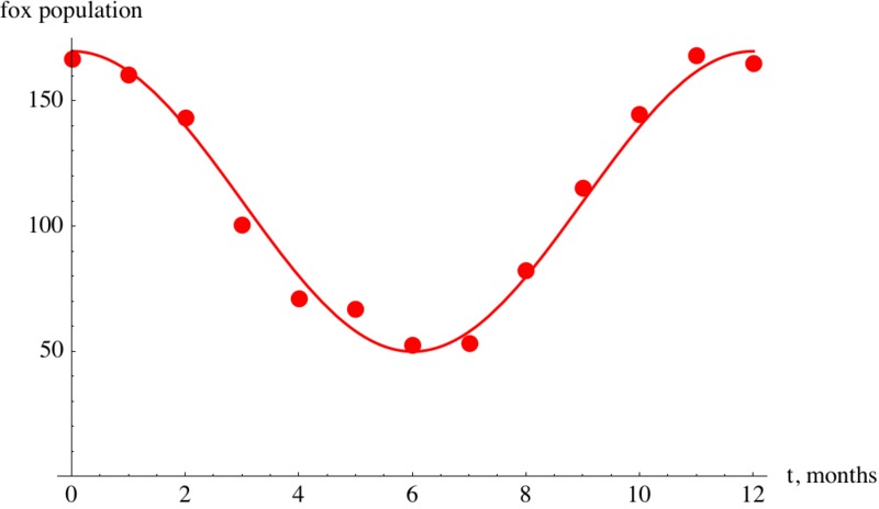
3. Again, we have to decide if we want to use sine or cosine to model this function. Looking at the graph, we observe that the fox population has a vertical intercept at its maximum and then decreases. This suggests the use of the cosine function $r(t) = A \cos(B(t - D)) + C$, where $A$ is the amplitude, $B = \frac{2 \pi}{\text{period}}$, $C$ is the midline, and the horizontal shift $D = 0$. From the graph, we estimate the minimum value to be 50 foxes and the maximum value to be 170 foxes. This gives us $A = (170 - 50)/2 = 60$, $C = (170 + 50)/2 = 110$ and $B = \frac{2\pi}{\text{period}} = \frac{2\pi}{12}$ , and we have $f(t) = 60 \cos( \frac{\pi}{6} t) + 110$.

   Graphing $f(t)$ together with our data points confirms that our function is a good model for the given data, if not perfect.